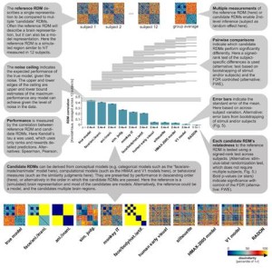
Hamed Nili, Nikolaus Kriegeskorte, and collaborators have published a toolbox for representational similarity analysis and an accompanying paper in PLoS Computational Biology. The toolbox enables anyone familiar with Matlab to test computational theories of brain information processing. It also introduces three new features of the method. The first new feature is the linear-discriminant t value, a measure of multiv ariate separation that bridges the gap between linear decoding and representational similarity analysis. The second new feature, detailed below, is the noise ceiling, which enables the user to assess which models fail to fully account for the data. The third new feature is an array of nonparametric inference techniques that can treat either the subjects or the stimuli, or both, as random effects. These techniques support generalisation to the population of people or stimuli. Representational similarity analysis is simple: Subjects are presented with a set of stimuli while their brain activity is measured. The representation in a given brain region is characterised by the dissimilarities between the response patterns. The dissimilarities indicate which distinctions are emphasised and which distinctions are deemphasised in the representation. Each computational model is given the same set of experimental stimuli to process. Its internal representation is then compared to the brain representation. If the two representations emphasize the same distinctions, the representational dissimilarity matrices (RDMs) of brain region and model representation will be correlated. The toolbox ranks all models by the degree to which they can account for the brain representation. Next, nonparametric inference techniques address three important questions: (1) Which models predict anything at all? (2) Which models does a given model beat (predicting significantly better)? (3) Which models fully explain the measurement of the representation? A model fully explains the data when its prediction accuracy hits the noise ceiling. Any remaining mismatch is then attributable to the noise in the measurements. When a model hits the ceiling, it’s time to stop working on the computational model and instead get better (or more) data, so as to reveal remaining deficiencies of the winning model.

 MRC Cognition and Brain Sciences Unit


